Logits Scales

Introduction

When I was learning how to use CNN to tackle the Carvana Competition on Kaggle, I came across with ENet that was used for Semantic Segmentation. I skimmed through a paper and looked at some sample code online, and I started writing my code for the ENet. If x is my input, then $z$=ENet($x$) is the set of logits I used for the calculation of the sigmoid cross entropy. I was not sure if I have made any mistakes in the codes, but using the Xavier initialization of the weights, the output $Z$ are really large - about $10^{40}$ or more. As ENet is composed of many "bottleneck" layers, I found out that after each pass of these bottleneck layers, the scale of the output is increased by a factor of 10. Thus, I tried to "manually" divide the output by 10 and the ENet finally kinda worked (far from perfectly, but at least the loss function is not NaN anymore and it is decreasing when training.

Because of this, I would like to investigate the effect of training and performance with different scales of logits using the famous MNIST data. (I cannot find anything online about this topics - but I think this is a very common question.)

Logistic Function $ y = \sigma(z) = \frac{1}{1+e^{-z}}$

The logistic function maps an input $z\in\mathbb{R}$ to $\sigma(z)\in (0,1)$. We can interpret $\sigma(z)$ as a probability of the unit being turned on, as the logit $\sigma(z)$ is between 0 and 1. Note that

$ f(0) = 0.5$
If $z<0 $, then $ \sigma(z) < 0.5$, which indicates that the unit is less likely to be turned on.
If $z>0 $, then $ \sigma(z) > 0.5$, which indicates that the unit is more likely to be turned on.

If we scale $z$ by a factor of $\alpha$, the above properties won't change. But the change of the probability will be more/less sensitive.

For example, let $z=1$. Then $\sigma(0.1z)\approx 0.52,\,\sigma(z)\approx 0.73$ and $ \sigma(10z)\approx 0.99995$. Note that a positive $z$ as above is interpreted as the unit being more likely to be turned on. The scale control "how" more likely. We can see that for $ \sigma(0.1z)$ it is just very slightly more likely, but for $\sigma(10z)$ it is super-duper likely that the unit is turned on. Refer to the graphs below.

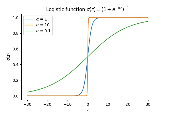
Thus scaling the logits $z$ changes the sensitivity of the output.

Softmax $ y = softmax(z)$

The softmax function $y = softmax(z)$ is a generalization of the above logistic function. Instead of thinking the unit being turned on and off, we say that $z$ can be in two states - "on" or "off". The sum of theprobability of the unit being "on" and the probability of the unit being "off" should be 1. Let $y_{on} = \sigma(z)$ be the logistic output of the logit $z$. Then we should have $y_{off} = 1 - \sigma(z)$. Note that $$y_{on}=\sigma(z) = \frac{1}{1+e^{-z}} = \frac{e^z}{e^z + 1} = \frac{e^z}{e^z + e^0}$$ and $$y_{off}= 1 - \sigma(z) = 1 - \frac{1}{1+e^{-z}} = \frac{e^{-z}}{1 + e^{-z}} = \frac{1}{e^z + 1} = \frac{e^0}{e^z + e^0}$$

Thus we can think of the input $z$ corresponds to $z_{on} = z$ and $z_{off} = 0$, with $$ y_{on} = \frac{e^{z_{on}}}{e^{z_{on}} + e^{z_{off}}}\mbox{ and } y_{off} = \frac{e^{z_{off}}}{e^{z_{on}} + e^{z_{off}}}$$

The advantage of this point of view is that if the output has several states, instead of just 2 (being either on or off), we can use the above formula to convert numbers into probabilities, such that a larger number of the state input corresponds to a larger probability of that state.

Let $z_i$ be the input of the $i$^th state and $y_i$ be the probabilities. Then we have $$ y_i = \frac{e^{z_i}}{\sum_j e^{z_j}} = \frac{e^{z_i}}{e^{z_1} + \ldots e^{z_n}} \quad\quad\mbox{(number of states}=n)$$

Let's do an example. Let's say there are 4 states such that $(z_1, z_2, z_3, z_4) = (2,2,4,-1)$. We can see that there state 1 and state 2 should happen equally likely, but state 3 is most likely to happen. We can use the above formulae to calculate the probabilities $y_i$ as below, $$e^{z_1} + e^{z_2} + e^{z_3} + e^{z_4} = e^2 + e^2 + e^4 +e^{-1}\approx 69.74$$ Thus $$y_1 \approx \frac{e^2}{69.74}\approx 0.106, \quad\quad y_2 \approx \frac{e^2}{69.74} \approx 0.106,\quad\quad y_3 \approx \frac{e^4}{69.74} \approx 0.783,\quad\quad y_4 \approx \frac{e^{-1}}{69.74}\approx 0.005$$

We can see that it agrees with our predictions. To simplify notation, we write $y = (y_1, \ldots, y_n)$ and $z=(z_1,\ldots, z_n)$ and $y = softmax(z)$. Note that both $y$ and $z$ are vectors here. We will still be referring $z$ as logits.

A nice property of softmax is that it is translation invariant, i.e. $softmax(z + C) = softmax(z)$. It can be easily shown as $$softmax(z+C) = \left(\frac{e^{z_i+C}}{\sum_j e^{z_j+C}}\right) = \left(\frac{e^{z_i}e^C}{\sum_j e^{z_j}e^C}\right) = \left(\frac{e^{z_i}}{\sum_j e^{z_j}}\right)=softmax(z)$$

Of course $C$ has to be the same across all states, i.e. $C$ is broadcasted to $z_j$.

Although the softmax function is translation invariant, it is not scale invariant. Again, just like the logistic function, it control the sensitivity of the probability output $y_i$. Using the example above, if $z = (2,2,4,1)$, then

$softmax(0.001z)\approx (0.25,0.25,0.25,0.25)$
$softmax(z) \approx(0.106,0.106,0.783,0.005)$
$softmax(0.5z) \approx (0.202,0.202,0.550,0.045)$
$softmax(2z) \approx (0.017,0.017,0.965,0)$
$softmax(10z) \approx (0,0,1,0)$

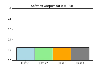
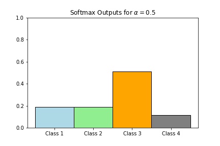
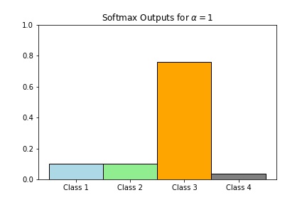
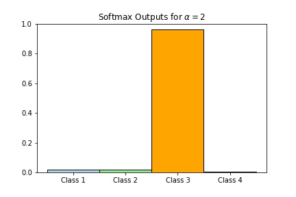
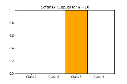
Scaling with a larger number will result in very close to hardmax (hence the name softmax) while scaling with a very small number will be close to the point where the states are all equally likely to happen.

Preliminary Analysis

After a short introduction, we can start with some theoretical analysis with the MNIST data. We let

$x$ - the input (`shape = [num_data, 784] or [num_data, 28,28]`).
$z = f(x;\theta)$ - the logits given parameters $\theta$ in a given network architecture $f$. (`z.shape = [num_data, 10]`)
$\hat{y} = softmax(z)$ - our prediction probability. (`shape = [num_data, 10]`)
$y$ - labels. (`shape = [num_data, 10]` after one-hot)

Then the loss function is given by $$L(x;\theta)=-\sum y_i \log \hat{y}_i$$

To reduce the loss, i.e. to train the model, we looked at the derivatives of $L$ with respect to $\theta$. We first have $$\dfrac{\partial L}{\partial z} =\hat{y}- y$$ (Here both $y$ and $z$ are vectors.) Thus by chain rules, we have $$\dfrac{\partial L}{\partial \theta} =(\hat{y} - y) \dfrac{\partial }{\partial \theta}\,f(x;\theta)$$ (Note that all of these are indeed vectors and matrices)

Now we are trying to scale the logits, i.e. let

$\hat{\tilde{y}} = softmax(\alpha z)$ for some $\alpha > 0$

We then have $$\dfrac{\partial \tilde{L}}{\partial z} =\alpha(\hat{\tilde{y}}- y)$$

This means $$\dfrac{\partial \tilde{L}}{\partial \theta} =\alpha(\hat{\tilde{y}} - y) \dfrac{\partial }{\partial \theta}\,f(x;\theta)$$

This means that if we scale our logits by a factor of $\alpha$, the gradient is also (apparently) scaled by a factor of $\alpha$. Of course it is not that simple, because if we scaled the logits, our probability vectors $\hat{y}$ changed and thus our losses also changed. It is very difficult to analyze how the training would turn out, but we can try to ignore the changes in our losses and just think that the gradient is just scaled by a factor of $\alpha$. Since we used the gradient for our learning, scaling the logits by a factor of $\alpha$ is similar to scaling our learning rate by a factor of $1/\alpha$, ignoring the (huge) possible effects of the changes in the loss function.

Note 1

In the most popular initializations of the weights $\theta$, the scaled logits $\alpha z$ (for large $\alpha$) may be very large and thus the loss function $L$ is also very large. This is because $$\log \hat{y}_i =\log \frac{e^{z_i}}{\sum_j e^{z_j}} =\log\frac{1}{1+\sum_{j\neq i} e^{z_j−z_i}} =−\log\left(1+\sum_{j\neq i} e^{z_j−z_i}\right)$$

When $z$ is replaced by $\alpha z$, we have $$\log \hat{\tilde{y}}_i = -\log\left(1+\sum_{j\neq i} e^{\alpha(z_j - z_i)}\right)$$

Assume that for some $\alpha(z_j - z_i)$ is positive and huge (say when $j=J$ ), then $$-\log\left(1+\sum_{j\neq i} e^{\alpha(z_j - z_i)}\right)\approx -\log e^{\alpha(z_J - z_i)} = -\alpha (z_J - z_i).$$

This means that if we adjusted our learning rate by the scale $\alpha$ (divided by $\alpha$ ), the decrease in $L$ would be small. Thus it should not be wise to adjust our learning rate when $\alpha$ is large.

Note 2

If $\alpha$ is small, then we have $$\log \hat{\tilde{y}}_i = -\log\left(1+\sum_{j\neq i} e^{\alpha(z_j - z_i)}\right) \approx -\log\left(1+\sum_{j\neq i} 1\right)\approx -\log 10$$ which is close to a constant. Thus $L$ very insensitive to changes. This seems to suggest that adjusting the learning rate is necessary. (Like dividing by $\alpha$

Note 3

It is anticipated the training would (hopefully) eventually train our scaled logits to a specific confortable range, no matter what $\alpha$ is. This is because if our initial prediction is incorrect, (if it is correct, why would we train?), then the logits must have to flip the sign (crossing 0). Thus if $\alpha$ is huge, after training the network for a while, we would expect our weights $\theta$ to be very small (hence our loss $L$ would fall into a desirable range). The unscaled logits $z$ will be small and $\alpha z$ would fall into the desired range. This means $\frac{\partial f}{\partial \theta}$ should stay in the same order of magnitude. If we adjust the learning rate as above, $L$ should decrease accordingly. This seems to suggest that for a large scale $\alpha$, we should adjust the learning rate in the beginning but we can adjust it after the scaled logits falls into the desired range.

Demo

After the above preliminary analysis, we are going to do some tests to see how the scaling of the logits would affect our training.

We are doing the followings,

We are using 98% of our data as training set and 2% of our data as test set.
We are investigating several archictecture including a fully connected net and three CNNs. We will be focusing on the fully connected set.

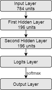
Fully Connected:

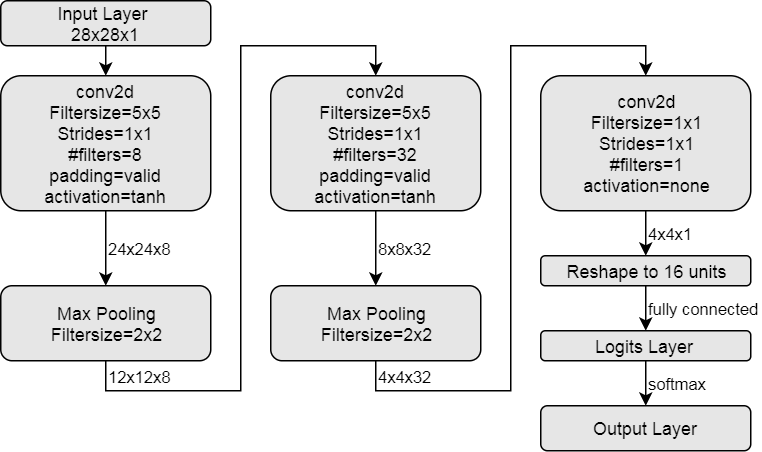
Convolutional Neural Network 1:

Convolutional Neural Network 2:

Convolutional Neural Network 3:
We are using Xavier initialization for the weights and zero initialization for the bias
Minibatch Size is 1024.
We will be keeping track of the standard deviation of the logits
You may wonder why the accuracy is very low compared to some other models training specifically for the MNIST data. We were just testing the scales of the logits, not aiming for very high accuracy of the model.

We will be testing different cases based on the followings,

We will be testing on 4 scale sets.
- A: $[0.1,0.3,1,3,10]$
- B: $[0.01,0.1,1,10,100]$
- C: $[10^{-8},10^{-6},10^{-4},10^{-1},1]$
- D: $[1,10^2, 10^4,10^6,10^8]$
Our base learning rates are $10^{-2}, 10^{-3}, 10^{-4}$ and $10^{-6}$.
We will try both adjusting the learning rates and not adjusting them.
We are using both gradient descent optimizer and Adam optimizer.
The number of epochs will be 10 and 50 for the fully connected network, and 10 for the CNNs.
We will interpret our result using a fixed random state 0. We also include results when the random state is None.

We ran this notebook on Kaggle Kernel.

Results

Our main graphs are based on Accuracy (in percent) on the test set vs Training time (logged every 3 minibatches).
We also logged the Standard Deviation of the Scaled Logits within a minibatch every 3 minibatches. These graphs are recorded starting from the 21st data points since the scales are too huge while not in logarithmic scale. An improvement would be outputing those in logarithmic scale - but we did not do it this time. Thus some of the graphs are pretty bad in scales.
We also include a training and test error as a percent of initial training and test error over 10 epochs.

Fully Connected

A Typical graph would be like below. Scale Set A Learning Rate = 0.001 Learning Rate Adjusted Gradient Descent Optimizer 50 Epochs Fixed Random State

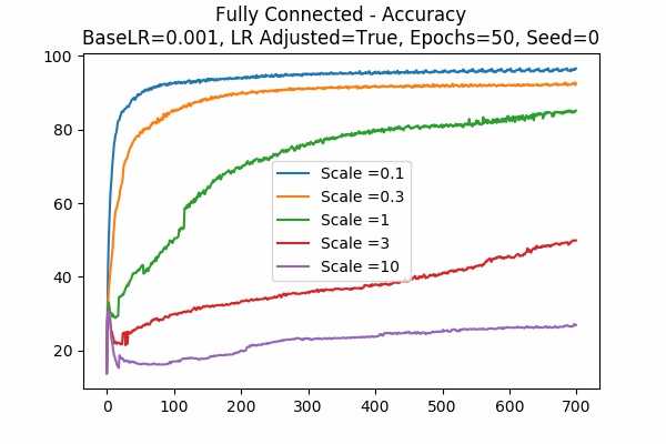
We can see that no scaling is not necessarily the best. Indeed here, we can see that the scale $\alpha = 0.1$ is the best.

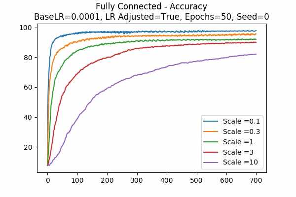
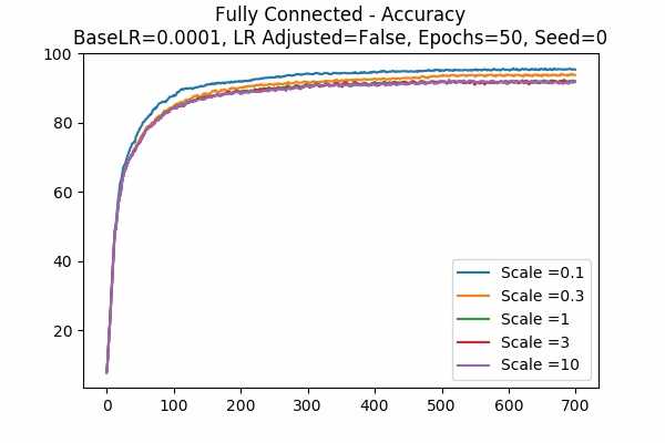
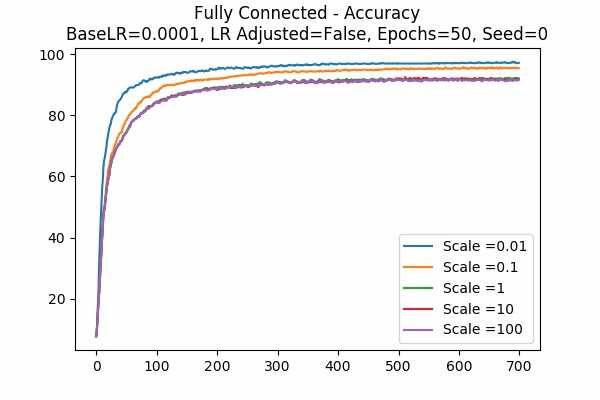
Some more graphs are shown below. Scale Set A Gradient Descent Optimizer 50 Epochs Fixed Random State

Learning Rate = 0.001 Learning Rate = 0.0001

Learning Rate Adjusted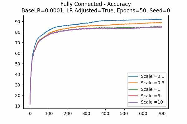

Learning Rate Unadjusted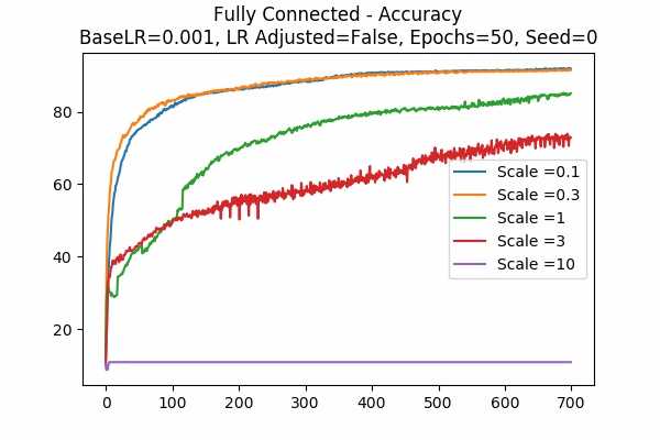

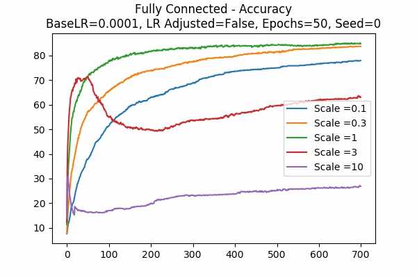
We can see that with learning rate as 0.001 and adjusted, a scale of 0.1 yields the best result after 50 epochs. It is interesting to see larger scales would yield the worst result by basically collapsing the accuracy. It also seems like adjusted learning rate would yield a better result.

Scale Set B Gradient Descent Optimizer 50 Epochs Fixed Random State

Learning Rate = 0.001 Learning Rate = 0.0001

Learning Rate Adjusted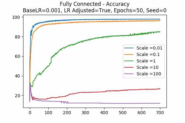

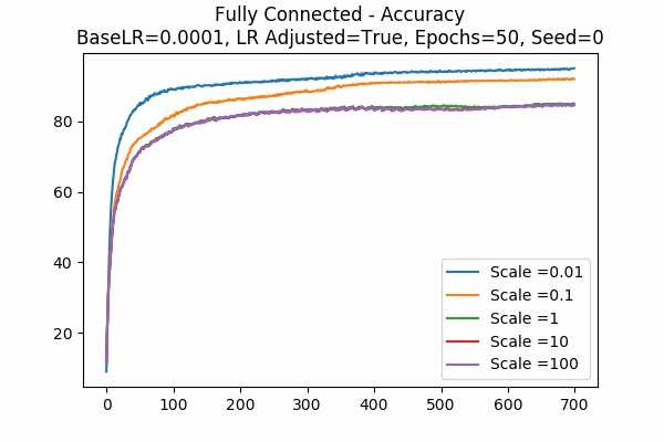
Learning Rate Unadjusted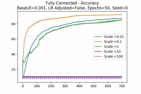

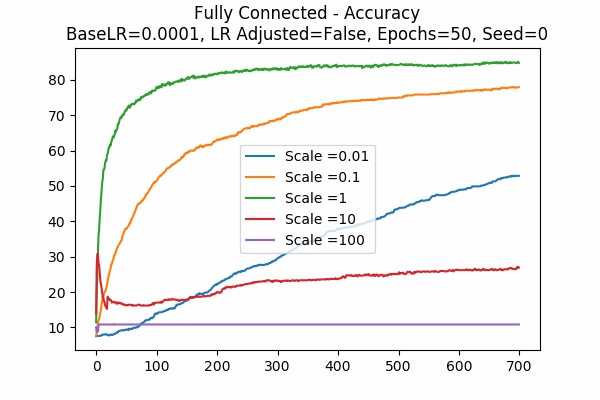
Since scale=0.1 is the best in the previous graphs, we looked at 0.01. Wow, when the learning rate is adjusted, they give the best results. While the learning rate is unadjusted, seems like 0.01 is a little to small. Again large scales usually yield very bad results unless we tune down the learning rate.

Scale Set A Adam Optimizer 50 Epochs Fixed Random State

Learning Rate = 0.001 Learning Rate = 0.0001

Learning Rate Adjusted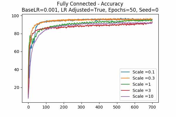

Learning Rate Unadjusted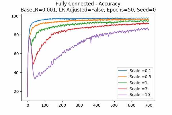

This is for the Adam Optimizer. Note that it is similar to the Gradient Descent Optimizer, but it performed a little bit better. Note that the graph for unadjusted learning rate with a base learning rate of 0.001, we see that when the scale is 10, the accuracy goes down very quickly and then slowly increases. This can be a phenomenon of setting the learning rate too high, while sometimes there will be exploding gradients. Luckily it was not too high so that the accuracy cannot recover. This agrees with our prediction that setting the logit scale higher will be similar to scaling the learning rate.

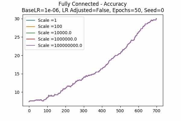
This graph is kinda interesting. Scale Set A Learning Rate = 0.000001 Learning Rate Unadjusted Gradient Descent Optimizer 50 Epochs Fixed Random State

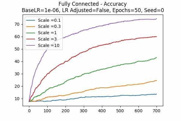
Note that if the learning rate is small, scaling the logits will help the training - however, we don't know what the endgame would be - and we cannot tune it down afterwards as all the weights $\theta$ are very much different. (Or can we? I don't know)

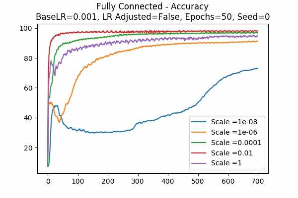
To see if our observation in Note 2 is correct. Scale Set C Learning Rate = 0.0001 Learning Rate Adjusted Gradient Descent Optimizer 50 Epochs Fixed Random State

It seems like what we predicted was true up until our learning rate is $10^{-8}$. Note that there are some gradient explosion on $10^{-6}$.

More... Scale Set C Learning Rate = 0.001 Learning Rate Unadjusted Adam Optimizer 50 Epochs Fixed Random State

This is a mystery of the Adam Optimizer. While the gradient descent counterpart agreed with our prediction on Note 2. The Adam Optimizer changes everything..

More... Scale Set B Adam Optimizer 50 Epochs Fixed Random State

Learning Rate = 0.001 Learning Rate = 0.0001

Learning Rate Adjusted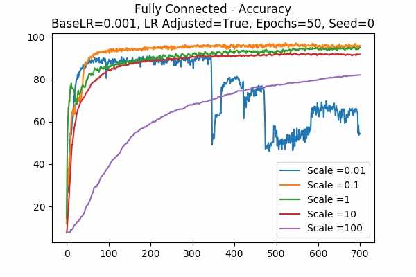

Learning Rate Unadjusted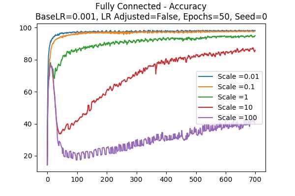

For the Adam Optimizer, it is interesting that in some cases, the accuracy went up at a peak but that plunges. This can be explained because the learning rate is high. For example if the learning rate is adjusted, a small scale would trigger the effect. Similarly, if the learning rate is unadjusted, a large scale would trigger the effect because again, scaling the logits is similar to scaling the learning rate.

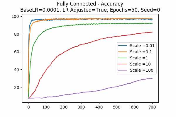
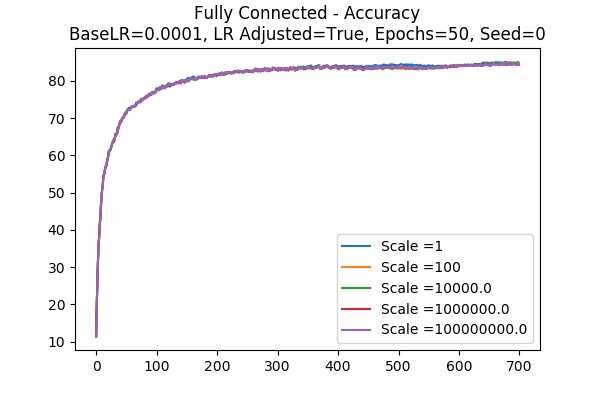
The following graphs are very surprising! Scale Set D Learning Rate = 0.0001 Learning Rate Adjusted Gradient Descent Optimizer 50 Epochs Fixed Random State

Note that for Gradient Descent Optimizer, this phenomenon agrees on what we said - scaling the logits is similar to scaling the learning rate. Since we adjusted the learning rate, the trend in accuracy should be similar. But it seems to only work for this base learning rate (0.0001)
Scale Set D Learning Rate Unadjusted Adam Optimizer 50 Epochs Fixed Random State

Learning Rate = 0.0001 Learning Rate = 0.000001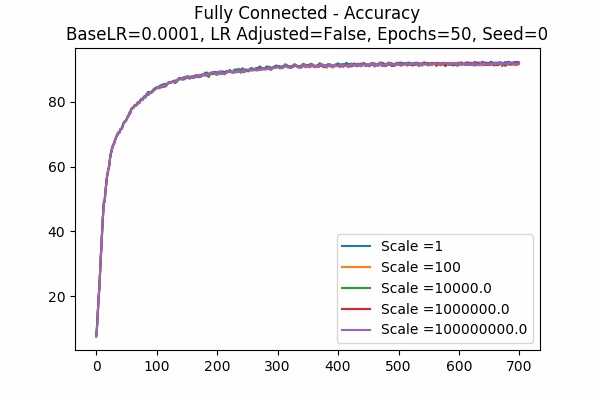

The phenomenon occurs again but with Adam Optimizer and Unadjusted learning rate. This is very surprising and it disagrees with what we think it would heppen. Does it have something to do with the memory of the Adam Optimizer? Or maybe the learning rate is automatically adjusted by the Optimizer? Maybe it is because of what we said in Note 1?

The followings are some comparisons.
- Random States Comparison Scale Set A Learning Rate = 0.001 Learning Rate Adjusted Gradient Descent Optimizer 10 Epochs
  
  Fixed Random State Random State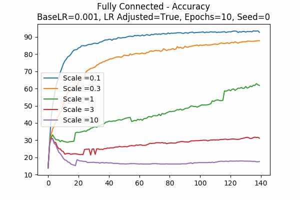
  
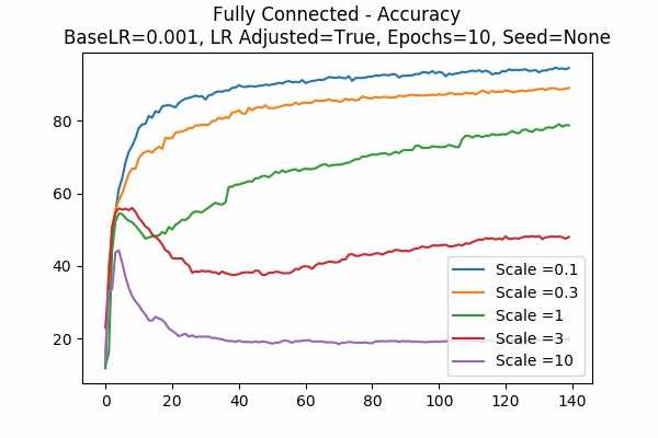
  It is clear that different optimization does make a huge difference in some of the cases. Of course if the random state is not fixed, the graph can be anything. The graph on the right hand side is just one of the many randomness.
- Optimizer Comparison Scale Set A Learning Rate Adjusted 50 Epochs Fixed Random State
  
  Learning Rate = 0.001 Learning Rate = 0.0001
  
  Gradient Descent Optimizer
  
  Adam Optimizer
  
  We can see that in both cases, Adam Optimizer performs better, which is not a surprise.
- Other Comparisons Scale Set B Learning Rate Adjusted Gradient Descent Optimizer 50 Epochs Fixed Random State
  
  Learning Rate = 0.001 Learning Rate = 0.0001
  
  We are looking at Scale = 0.1 on the left and Scale = 0.01 on the right. Note that they have the same adjusted learning rate - $ \frac{0.001}{0.1} = \frac{0.0001}{0.01} = 0.01$. Note that both lines are very similar.
  However, for Scale = 1 on the left and Scale = 0.1 on the right, even though they have the same adjusted learning rate, they are pretty different. This can be seen in other cases in the above graphs.
- Similar for Adam... Scale Set B Learning Rate Adjusted Adam Optimizer 50 Epochs Fixed Random State
  
  Learning Rate = 0.001 Learning Rate = 0.0001
  
  We are doing the above comparisons for the Adam Optimizer. Note that most of them are not similar except for Scale = 100 on the left and Scale = 10 on the right and Scale = 10 on the left and Scale = 1 on the right
- But things worked out in the following case for Adam. Scale Set B Learning Rate Adjusted Adam Optimizer 50 Epochs Fixed Random State
  
  Learning Rate = 0.0001 Learning Rate = 0.000001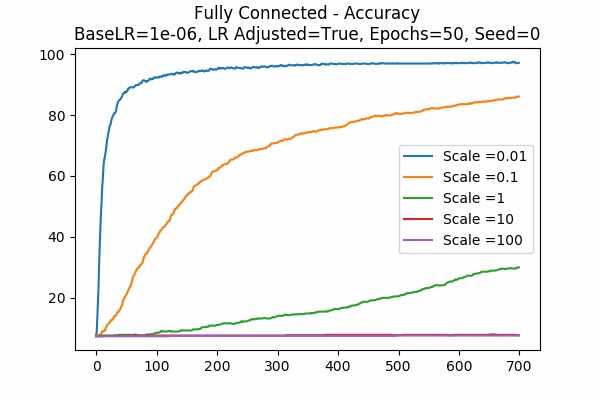
  
  Note that if we compare the above 2 graphs for really small base learning rates, all the accuracies for the same agreed adjusted learning rates match. This includes
  - Scale = 1 on the left and Scale = 0.01 on the right. (Adjusted Learning Rate = 0.0001)
  - Scale = 10 on the left and Scale = 0.1 on the right. (Adjusted Learning Rate = 0.00001)
  - Scale = 100 on the left and Scale = 1 on the right. (Adjusted Learning Rate = 0.000001)
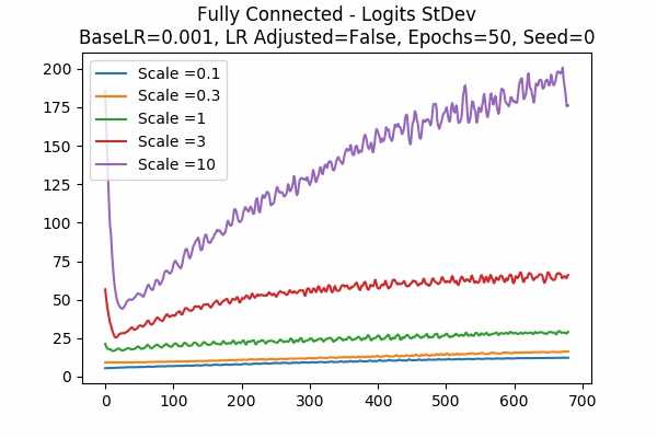
We want to know for what learning rates and what scales would yield the best results. So we are looking at the spread for the logits. Our prediction was that at all scales, if the model is training well, the range of the logits should fall into an acceptable range. We can see below. Scale Set A Learning Rate = 0.001 Learning Rate Adjusted Gradient Descent Optimizer 50 Epochs Fixed Random State

Accuracy StDev: Scaled Logits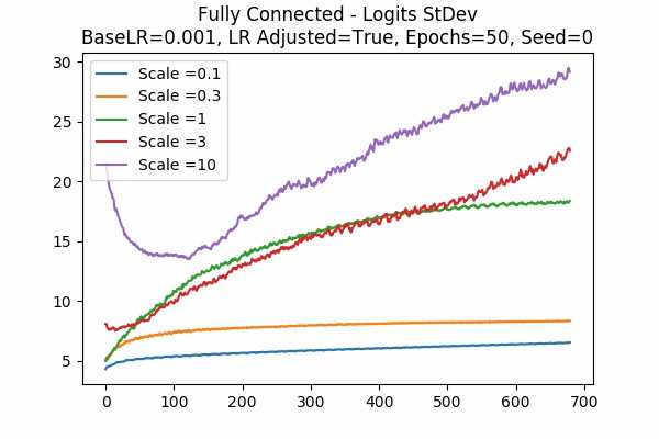

Note that for the better models, the StDev of the scaled logits are about 2.5 to 20. For larger scales, the StDev first decreases, then increases again (which is imaginable after training for a longer time). It is clear that the initial StDev of the logits are exactly proportional to the scale because we fixed the random seed. Recall that our graphs start at the 21st data points for the StDev.
Scale Set B Learning Rate = 0.001 Learning Rate Unadjusted Gradient Descent Optimizer 50 Epochs Fixed Random State

Accuracy StDev: Scaled Logits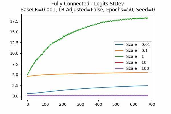

Still True. 2.5 to 20. Even for very small scales like 0.01.
Scale Set C Learning Rate = 0.001 Learning Rate Unadjusted Adam Optimizer 50 Epochs Fixed Random State

Accuracy StDev: Scaled Logits

This is the strongest graph that shows that the logit ranges should fall into an acceptable region. Note that the initial StDev is very small because of the very small scales we put here. Although for Set D it is no longer true - although the StDev keeps decreasing and gap between scaled logits of different scales become smaller. (We did not put the graphs here because it is not in logarithmic scale. You can see these here)
Scale Set B Learning Rate = 0.0001 Learning Rate Unadjusted Gradient Descent Optimizer 50 Epochs Fixed Random State

Accuracy StDev: Scaled Logits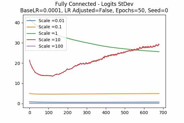

This is a different learning rate (0.0001). Note that still the scaled logits of the better models are converging to the range between 2.5 to 20(ish).

Scaled Logits StDev Comparison of Gradient Descent and Adam Optimizer Learning Rate = 0.001 Learning Rate Unadjusted 50 Epochs Fixed Random State

Gradient Descent Optimizer Adam Optimizer

Scale Set A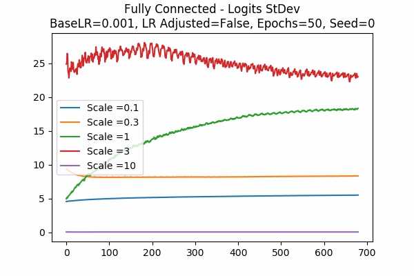

Scale Set B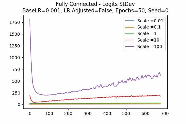

Since Adam Optimizer is usually the optimizer we used, we are looking at the StDev of the scaled logits. We can see that the range is not 2.5 to 20 anymore, but it is much larger. Would it be the case that using Adam Optimizer, the prediction is good already and they wanted to make it closer to a hardmax?

Training Error and Test Error. Scale Set A Learning Rate Adjusted Adam Optimizer 10 Epochs Fixed Random State

Learning Rate = 0.001 Learning Rate = 0.00001

Training Error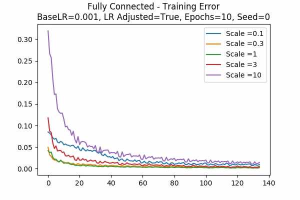

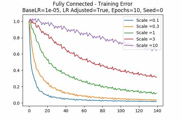
Test Error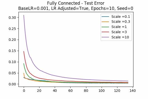

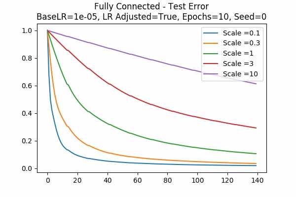
We just include the training and test error here, for two different learning rate (a new learning rate 1e-5!) Note that the y-axis denotes the percentage of the initial error. For learning rate = 0.001, because the error decreases very quickly, we started at the 6th data points. Note that in both cases, because the learning rate is adjusted, the error is decreased more slowly for large scales.

Convolutional Neural Networks

Since the training time is much longer for our CNN models, we are just run 10 epochs and we just have a few graphs shown below.

Type 1

A Typical graph would be like below. Scale Set A Learning Rate = 0.001 Learning Rate Adjusted Adam Optimizer 10 Epochs Fixed Random State

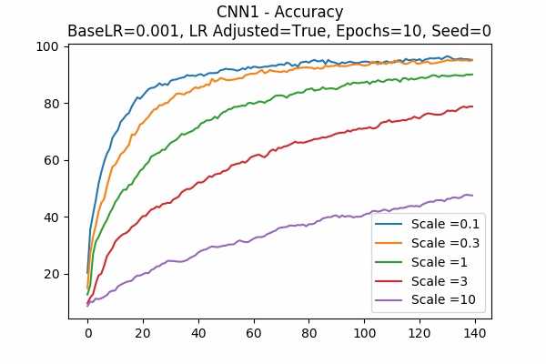
We can see that the learning time is greatly affected by the scale. We can either not adjust the learning rate, or increase the base learning rate.

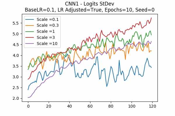
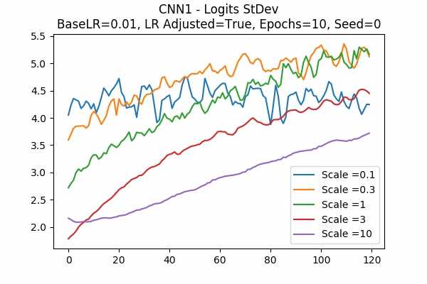
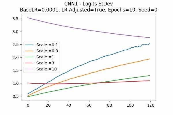
These are the deviations from the above graphs Scale Set A Learning Rate = 0.001 Learning Rate Adjusted Adam Optimizer 10 Epochs Fixed Random State

	Accuracy	Scaled Logits StDev
Original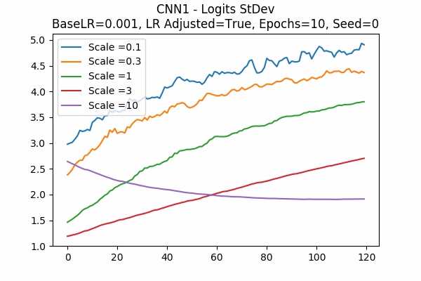
Learning Rate = 0.1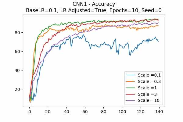
Learning Rate = 0.01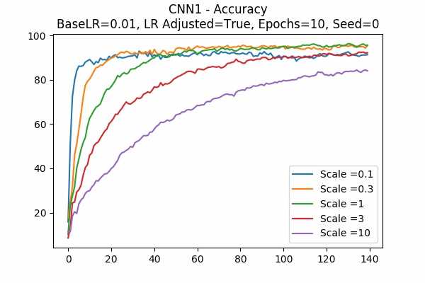
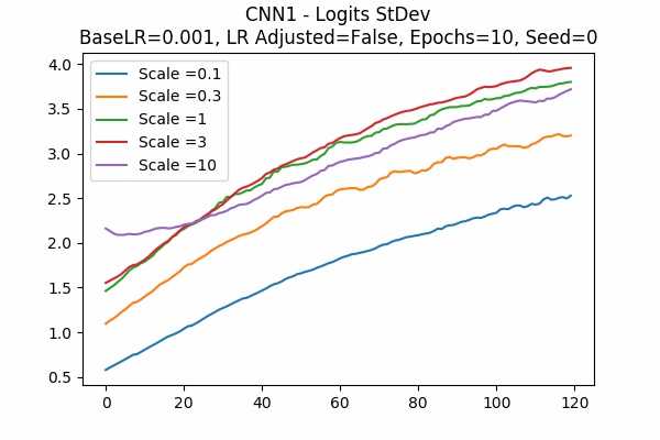
Learning Rate = 0.0001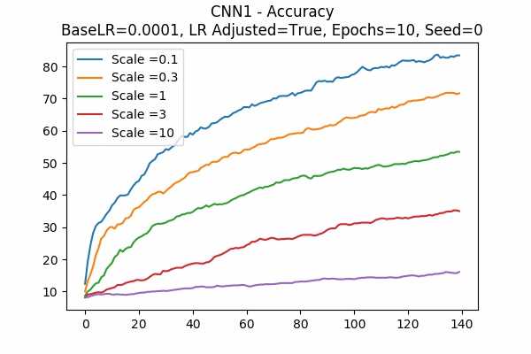
Learning Rate Unadjusted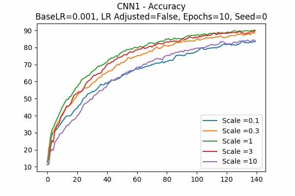
Scale Set B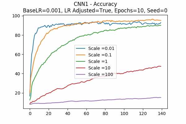

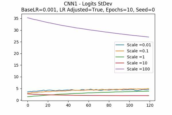
It is interesting that for Scale Set A, the standard deviation of the logits are mainly in a comfortable range regardless of the scales. It is met with an example of bad range with a bad result in Scale Set B. (Scale = 100)
It also confirms the above mentioned suggestion - the accuracy increases when we increase the learning rate or not to adjust the learning rate.

Type 2

A Typical graph would be like below. Scale Set A Learning Rate = 0.01 Learning Rate Adjusted Adam Optimizer 10 Epochs Fixed Random State

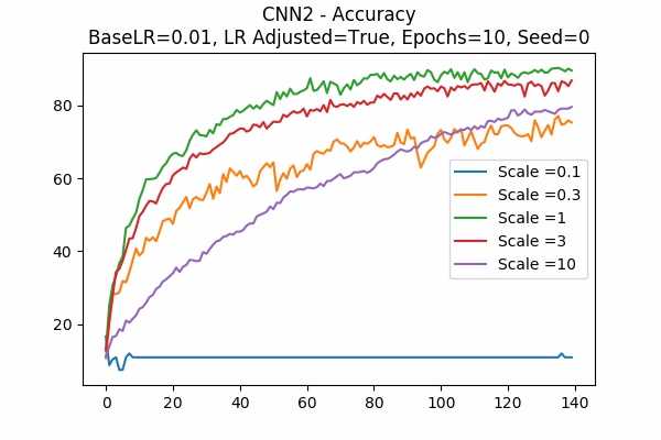
For this CNN model, it seems that a learning rate of 0.01 is too huge so that a smaller scale of 0.1 with learning rate adjusted does not work.

These are the deviations from the above graphs Scale Set A Learning Rate = 0.01 Learning Rate Adjusted Adam Optimizer 10 Epochs Fixed Random State

Accuracy Scaled Logits StDev

Original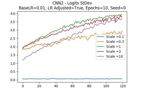

Learning Rate = 0.001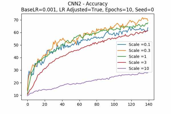

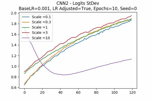
Learning Rate Unadjusted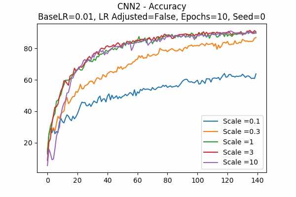

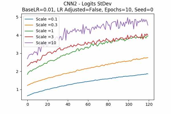
Scale Set B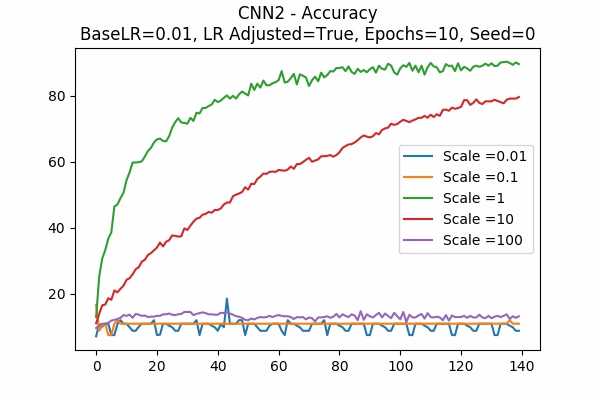

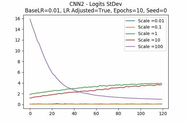
Random State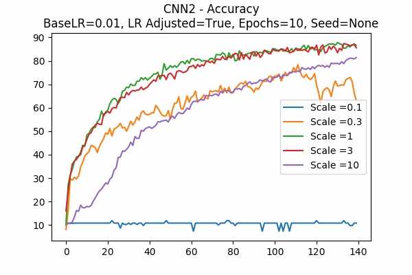

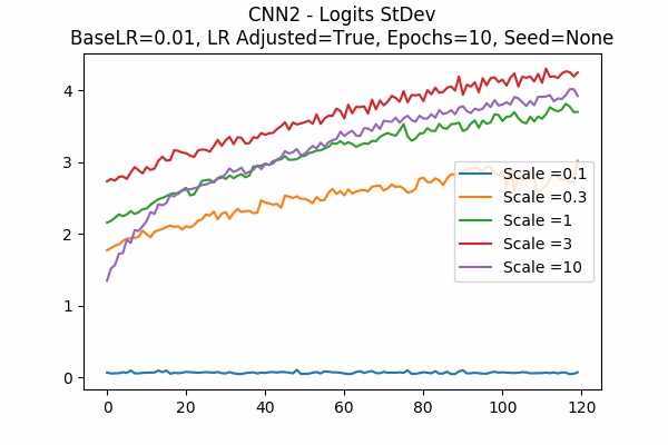
The surprising thing is that the scaled logits for scale = 0.1 are very small either. It seems not adjusting the learning rate would be better. Note that in this model, it seems that no scaling would do the job. The scaled logits are also in a comfortable range.

Type 3

A Typical graph would be like below. Scale Set A Learning Rate = 0.01 Learning Rate Adjusted Adam Optimizer 10 Epochs Fixed Random State

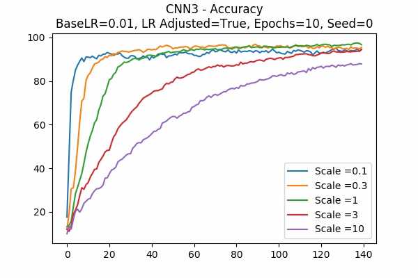
It seems like this model works a lot better than the last one.

These are the deviations from the above graphs Scale Set A Learning Rate = 0.01 Learning Rate Adjusted Adam Optimizer 10 Epochs Fixed Random State

Accuracy Scaled Logits StDev

Original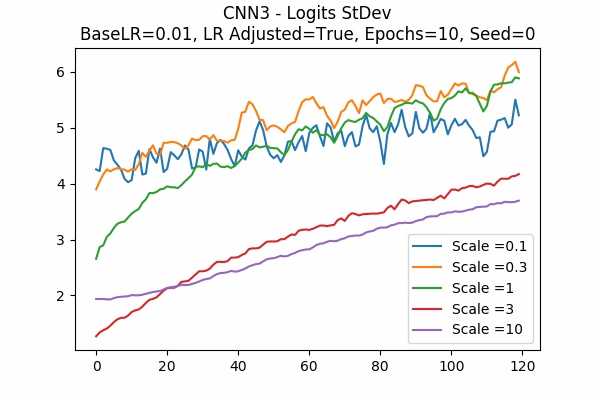

Learning Rate = 0.001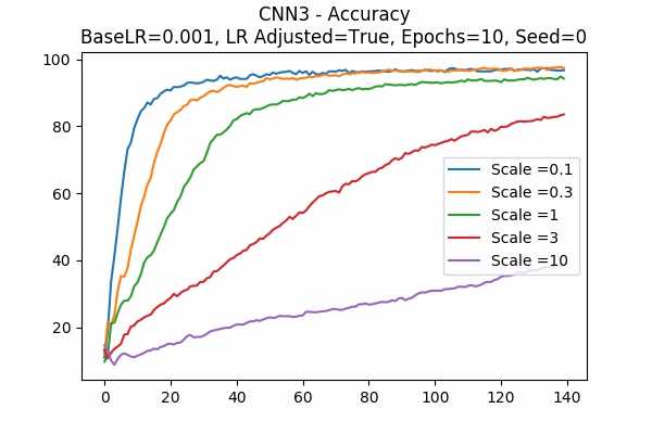

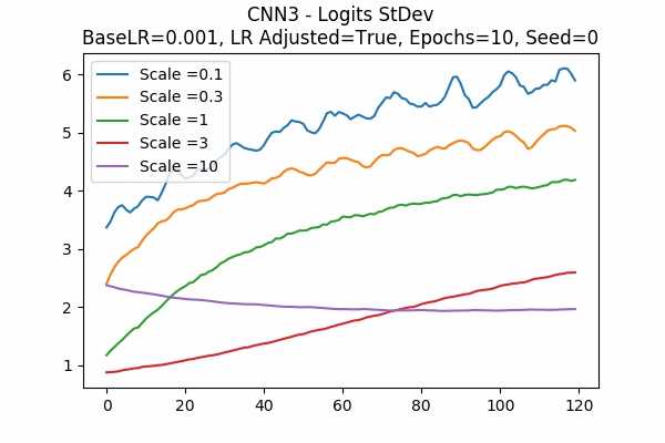
Learning Rate Unadjusted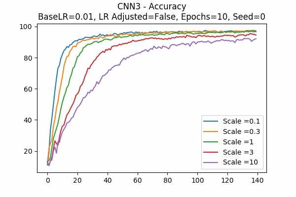

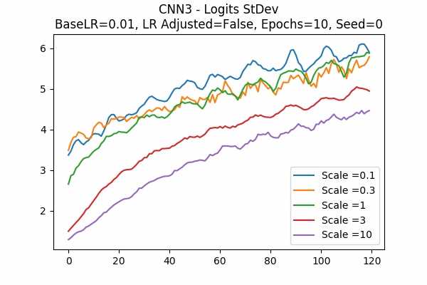
Scale Set B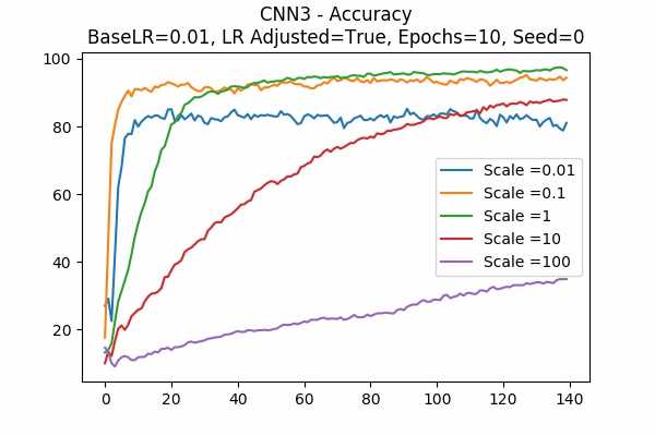

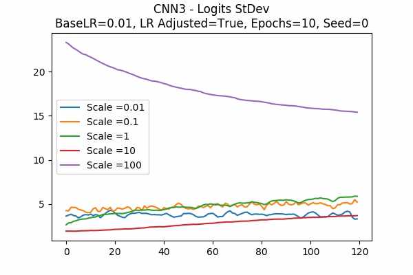
Random State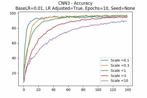

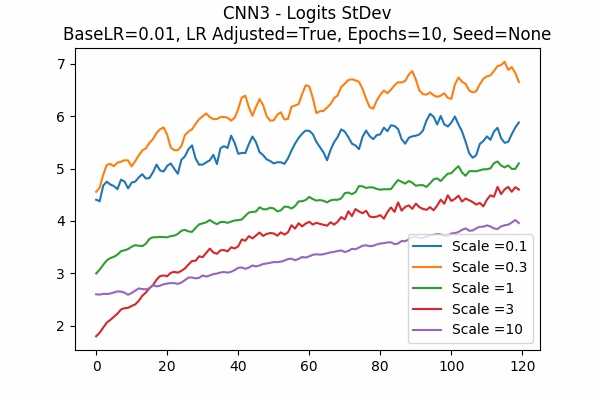
I am surprised that none failed. Even all scales in Scale Set B.

Conclusion

We can say with some (vague) statements.

Logit Scales do affect our model and training. It seems to me that before training, one should check the logits with your favourite weights initialization method, and scale it down accordingly, instead of using the weights to do the work. c.f. normalizing the units to have mean 0 and variance 1 instead of not doing it and let the bias trained.
It is a hyperparameter which correlates very closely to the learning rate. For some cases they are highly correlated
It works differently for Gradient Descent Optimizer and Adam Optimizer. (Duh!)
Of course it depends greatly of your model (Duh!)

Code

Code (Python)


import numpy as np
import pandas as pd
import matplotlib.pyplot as plt
import tensorflow as tf
import time
from sklearn.model_selection import train_test_split
from sklearn.preprocessing import OneHotEncoder
df = pd.read_csv('../input/train.csv')	  
Xtrain, Xtest, ytrain, ytest = train_test_split(df.iloc[:,1:],
                                                df.iloc[:,0],
                                                train_size=0.98, 
                                                test_size=0.02, 
                                                random_state=0)
Xtrain=np.array(Xtrain).reshape(-1,28,28,1)
Xtest=np.array(Xtest).reshape(-1,28,28,1)
enc = OneHotEncoder()
ytrain= enc.fit_transform(np.array(ytrain).reshape(-1,1)).toarray()
ytest= enc.transform(np.array(ytest).reshape(-1,1)).toarray()	  
	  
#Several network architecture. the input x is the input placeholder and return a logit tensor.
def fc(x):
    n_train = tf.shape(x)[0]
    net = tf.reshape(x, [n_train, 784])
    net = tf.contrib.layers.fully_connected(net, 196, activation_fn=tf.nn.relu)
    net = tf.contrib.layers.fully_connected(net, 49, activation_fn=tf.nn.relu)
    return tf.contrib.layers.fully_connected(net, 10, activation_fn=None)

def cnn1(x):
    net = tf.layers.conv2d(x,8,[5, 5],strides=(1,1),padding="valid",activation=tf.tanh)
    net = tf.layers.max_pooling2d(inputs=net, pool_size=[2, 2], strides=2)
    net = tf.layers.conv2d(net,32, [5,5], strides=(1,1), padding="valid", activation=tf.tanh)
    net = tf.layers.max_pooling2d(inputs=net, pool_size=[2, 2], strides=2)
    net = tf.layers.conv2d(net,1, [1,1], strides=(1,1), padding="same", activation=None)
    n_train = tf.shape(net)[0]
    net = tf.reshape(net, [n_train, 16])
    return tf.contrib.layers.fully_connected(net, 10, activation_fn=None)

def cnn2(x):
    net = tf.layers.conv2d(x , 4, [5,5], strides=(1,1), padding="valid", activation=tf.tanh)
    net = tf.layers.conv2d(net,4, [5,5], strides=(1,1), padding="valid", activation=tf.tanh)
    net = tf.layers.conv2d(net,4, [5,5], strides=(1,1), padding="valid", activation=tf.tanh)
    net = tf.layers.conv2d(net,4, [5,5], strides=(1,1), padding="valid", activation=tf.tanh)
    net = tf.layers.conv2d(net,4, [5,5], strides=(1,1), padding="valid", activation=tf.tanh)
    net = tf.layers.conv2d(net,4, [5,5], strides=(1,1), padding="valid", activation=tf.tanh)
    net = tf.layers.conv2d(net,1, [1,1], strides=(1,1), padding="valid", activation=tf.tanh)
    n_train = tf.shape(net)[0]
    net = tf.reshape(net, [n_train, 16])
    return tf.contrib.layers.fully_connected(net, 10, activation_fn=None)

def cnn3(x):
    net = tf.layers.conv2d(x,16,[3, 3],strides=(1,1),padding="valid",activation=tf.tanh)
    net = tf.layers.max_pooling2d(inputs=net, pool_size=[2, 2], strides=2)
    net = tf.layers.conv2d(net,64, [4,4], strides=(1,1), padding="valid", activation=tf.tanh)
    net = tf.layers.max_pooling2d(inputs=net, pool_size=[2, 2], strides=2)
    net = tf.layers.conv2d(net,1, [1,1], strides=(1,1), padding="same", activation=None)
    n_train = tf.shape(net)[0]
    net = tf.reshape(net, [n_train, 25])
    return tf.contrib.layers.fully_connected(net, 10, activation_fn=None)	  

def runnet(Xtrain, Xtest, ytrain, ytest, 
           func,
           epochs = 5,
           scale = 1, 
           base_lr = 0.001, 
           learning_rate_adjusted = False, 
           op = 'GD',
           seed=None):
    #Check Validity of the above defined functions
    if func not in [cnn1,cnn2,cnn3,fc]:
        print('Input Function Incorrect!')
        return
    if op not in ['GD','AD']:
        print('Optimizers are GradientDescentOptimizer ("GD") or AdamOptimizer ("AD")')
        return
    #Enable Reverse One-Hot By Multiplying numlist
    numlist=np.array([0,1,2,3,4,5,6,7,8,9])
    tf.reset_default_graph()
    tf.set_random_seed(seed)
    x = tf.placeholder(tf.float32, shape=[None, 28,28,1])
    y = tf.placeholder(tf.float32, shape = [None, 10])
    lr = tf.placeholder(tf.float32, shape = [])
    out = func(x) * scale #Scaled Logits
    loss=tf.reduce_mean(tf.nn.softmax_cross_entropy_with_logits(labels=y, logits=out))
    if op == 'GD':
        train_step = tf.train.GradientDescentOptimizer(lr).minimize(loss)
    elif op == 'AD':
        train_step = tf.train.AdamOptimizer(lr).minimize(loss)
    bs = 1024 #batch_size
    #For plotting purposes
    acclist=[] 
    stdlist=[]
    #trainlist=[]
    #testlist=[]
    if learning_rate_adjusted:
        rate = base_lr / scale 
    else:
        rate = base_lr
    with tf.Session() as sess:
        sess.run(tf.global_variables_initializer())
        #initial error
        er=sess.run(loss, feed_dict={x:Xtrain[:1], y:ytrain[:1], lr: 0})
        print('Running: Scale={}, BaseLR={}, LR_Adjusted={}, Seed={}, Optimizer={}'.format(
            scale, base_lr, learning_rate_adjusted, seed, op))
        print('Initial Logits StDev: ',np.std(sess.run(out, feed_dict={x:Xtest})))
        for i in range(epochs):
            tic = time.time()
            #ignore last incomplete batch
            for j in range(len(Xtrain)//bs):
                _, er=sess.run([train_step, loss], feed_dict={
                    x:Xtrain[j*bs:(j+1)*bs], 
                    y:ytrain[j*bs:(j+1)*bs], 
                    lr: rate})
                ertest, pred = sess.run([loss,out], feed_dict={x:Xtest, y:ytest})
                stdev = np.std(pred)
                #Prediction Before Reverse One-Hot
                pred=np.argmax(pred, axis=1)
                #Accuracy of Prediction After Reverse One-Hot
                acc=(pred==np.dot(ytest, numlist)).sum()/len(ytest)*100
                if j%3==0:
                    #print('Training Error: {:8.4f}\tTest Error: {:8.4f}\tAccuracy: {:5.2f}%'.format(er, ertest, acc))
                    acclist.append(acc)
                    stdlist.append(stdev)
                    #trainlist.append(er)
                    #testlist.append(ertest)
            toc = time.time()
            print('Epoch {}\tTraining Error: {:8.4f}\tTest Error: {:8.4f}\tAccuracy: {:5.2f}%\tTime: {:6.2f}s'.format(
                i+1,er, ertest, acc, toc- tic))
            tic = toc
    return acclist, stdlist#, trainlist, testlist

lrlist = [1e-2,1e-3,1e-4,1e-6]
bstr = ["1e-2","1e-3","1e-4","1e-6"]
scalelistlist = [[0.1,0.3,1,3,10],[0.01,0.1,1,10,100],[1e-8,1e-6,1e-4,1e-2,1],[1,100,1e4,1e6,1e8]]
sstr = ["A","B","C","D"]
#[0.1,0.3,1,3,10] #A
#[0.01,0.1,1,10,100] #B
#[1e-8,1e-6,1e-4,1e-2,1] #C
#[1,100,1e4,1e6,1e8] #D
op = "GD"
ep=10
adj=True
sd=0
for j in range(4):
    for k in range(4):
        ACC = []
        STD = []
        base_lr = lrlist[j]
        scalelist = scalelistlist[k]
        for scale in scalelist:
            acclist, stdlist = runnet(Xtrain, Xtest, ytrain, ytest, 
                                      fc, 
                                      base_lr=base_lr,
                                      epochs = ep,
                                      scale=scale,
                                      learning_rate_adjusted = adj,
                                      op='GD',
                                      seed=sd)
            ACC.append(acclist)
            STD.append(stdlist)
        plt.title('Fully Connected - Accuracy\nBaseLR={}, LR Adjusted={}, Epochs={}, Seed={}'.format(
            base_lr,adj,ep,sd))
        for i in range(len(ACC)):
            if len(ACC[i])>0:
                plt.plot(ACC[i], label='Scale ='+str(scalelist[i]))
        plt.legend()
        plt.show()
        plt.title('Fully Connected - Logits StDev\nBaseLR={}, LR Adjusted={}, Epochs={}, Seed={}'.format(
            base_lr,adj,ep,sd))   
        for i in range(len(STD)):
            if len(STD[i][20:])>0:
                plt.plot(STD[i][20:], label='Scale ='+str(scalelist[i]))
        plt.legend()
        plt.show()

Kin Kwan Leung

Zillow

Logits(current)

Carvana

CV

Contact

Introduction

Logistic Function \( y = \sigma(z) = \frac{1}{1+e^{-z}}\)

Softmax \( y = softmax(z)\)

Preliminary Analysis

Note 1

Note 2

Note 3

Demo

Results

Fully Connected

Convolutional Neural Networks

Type 1

Type 2

Type 3

Conclusion

Code

Code (Python)

	Learning Rate = 0.001	Learning Rate = 0.0001
Learning Rate Adjusted
Learning Rate Unadjusted

	Learning Rate = 0.001	Learning Rate = 0.0001
Gradient Descent Optimizer
Adam Optimizer

	Gradient Descent Optimizer	Adam Optimizer
Scale Set A
Scale Set B

	Learning Rate = 0.001	Learning Rate = 0.00001
Training Error
Test Error

Kin Kwan Leung Zillow Logits(current) Carvana CV Contact

Introduction

Logistic Function \( y = \sigma(z) = \frac{1}{1+e^{-z}}\)

Softmax \( y = softmax(z)\)

Preliminary Analysis

Note 1

Note 2

Note 3

Demo

Results

Fully Connected

Convolutional Neural Networks

Type 1

Type 2

Type 3

Conclusion

Code

Code (Python)

Kin Kwan Leung

Zillow

Logits(current)

Carvana

CV

Contact